Distribution Functions
Overview
There are many existing packages designed to learn Gaussian Mixture Models, for example for clustering.
However, there are relatively few that provide a simple interface to compute the common distribution functions of a Gaussian mixture such as the PDF and CDF given a known set of model parameters.
The module gmix2 implements the following methods:
- probability density function
- cumulative distribution function
- percent point function (aka quantile or inverse cumulative distribution function)
- mean
- median
- mode(s)
- random values using inverse transform sampling.
IMPORTANT - All numpy arrays must be created using the ‘C’ / row major storage order, which should be the default.
Examples
The examples below all assume the following variables describing two univariate Gaussian mixtures.
>>> import numpy as np
>>> import gmix2 as gmix

# In these examples there are 2 distinct mixtures
# each composed of 5 Normal distributions. The distribution functions
# can compute the values for multiple mixtures with different parameters
# at once (as long as they have the same number of components). So,
# these functions expect the parameter arrays to be 2 dimensional of
# shape: (# mixture distributions, # Normals in mixture)

# Each Normal distribution in the mixture is characterized by its mean
# and variance.
>>> means = np.array([
    [ 0.0,  1.0, 2.0, 3.0, 4.0],
    [-5.0, -2.0, 0.0, 1.0, 3.0]
])

# These are the standard deviations of the distribution (not the
# variance).
>>> sigmas = np.array([
    [0.9,  0.5, 2.0, 1.0, 3.0],
    [0.5, 10.0, 2.0, 5.0, 0.8]
])

# Each Normal in the mixture is weighted by a value that sums to 1 over
# all the weights in the mixture.
>>> weights = np.array([
    [0.15, 0.10, 0.40, 0.05, 0.3],
    [0.05, 0.20, 0.10, 0.35, 0.3]
])
The gmix2.pdf
# The PDF of the two mixtures applied at the point 1.
>>> gmix.pdf(1, weights, means, sigmas)
array([0.21296355, 0.05973009])

# The PDF of the two mixtures applied at the point -5.5.
>>> gmix.pdf(-5.5, weights, means, sigmas)
array([0.00033562, 0.04415236])

# Unlike the original gmix, you can find the PDF of more than one value
# at a time. This operation is vectorized and very efficient compared
# to calculating each PDF separately.
>>> gmix.pdf([1.0, -5.5], weights, means, sigmas)
array([[0.21296355, 0.00033562],
       [0.05973009, 0.04415236]])
The gmix2.cdf
>>> gmix.cdf(1, weights, means, sigmas)
array([0.35216006, 0.41959143])

>>> gmix.cdf(-5.5, weights, means, sigmas)
array([0.00026666, 0.11474478])

>>> gmix.cdf([1, -5.5], weights, means, sigmas)
array([[0.352160058832, 0.000266662424],
       [0.419591430163, 0.11474477839]])
The gmix2.ppf
>>> gmix.ppf(0.3, weights, means, sigmas)
array([ 0.75333973, -1.18581628])

>>> gmix.ppf(0.9, weights, means, sigmas)
array([5.673111  , 5.91678309])

>>> gmix.ppf([0.3, 0.9], weights, means, sigmas)
array([[ 0.75333973,  5.673111  ],
       [-1.18581628,  5.91678309]])
The gmix2.mean
>>> gmix.mean(weights, means)
array([2.25, 0.6])
The gmix2.median
>>> gmix.median(weights, means, sigmas)
array([1.79712881, 2.00299055])
The gmix2.mode
# For each mixture this function will return a list of tuples
# corresponding to one or more modes (local maxima). The first value of
# the tuple is the x value of the mode and the second value is the pdf
# at that x value.
>>> gmix.mode(weights, means, sigmas)
[[(0.9580152000982137, 0.21324093573952826)],
 [(-4.970966372242318, 0.06205794913899075),
  (2.96872434469676, 0.189013117805071)]]
The gmix2.variance
>>> gmix.variance(weights, means, sigmas)
array([ 6.384 , 34.0945])
The gmix2.random
# Create a RandomState for reproducible results
>>> rng = np.random.RandomState(31)

# Generate 5 random numbers from each distribution
>>> gmix.random(5, weights, means, sigmas, rng)
array([[ 0.68525795,  7.31726575,  3.91860072,  9.13348322,  0.26170822],
      [-1.47038713,  9.38198888,  3.63405966, 13.83377875, -3.4449309 ]])
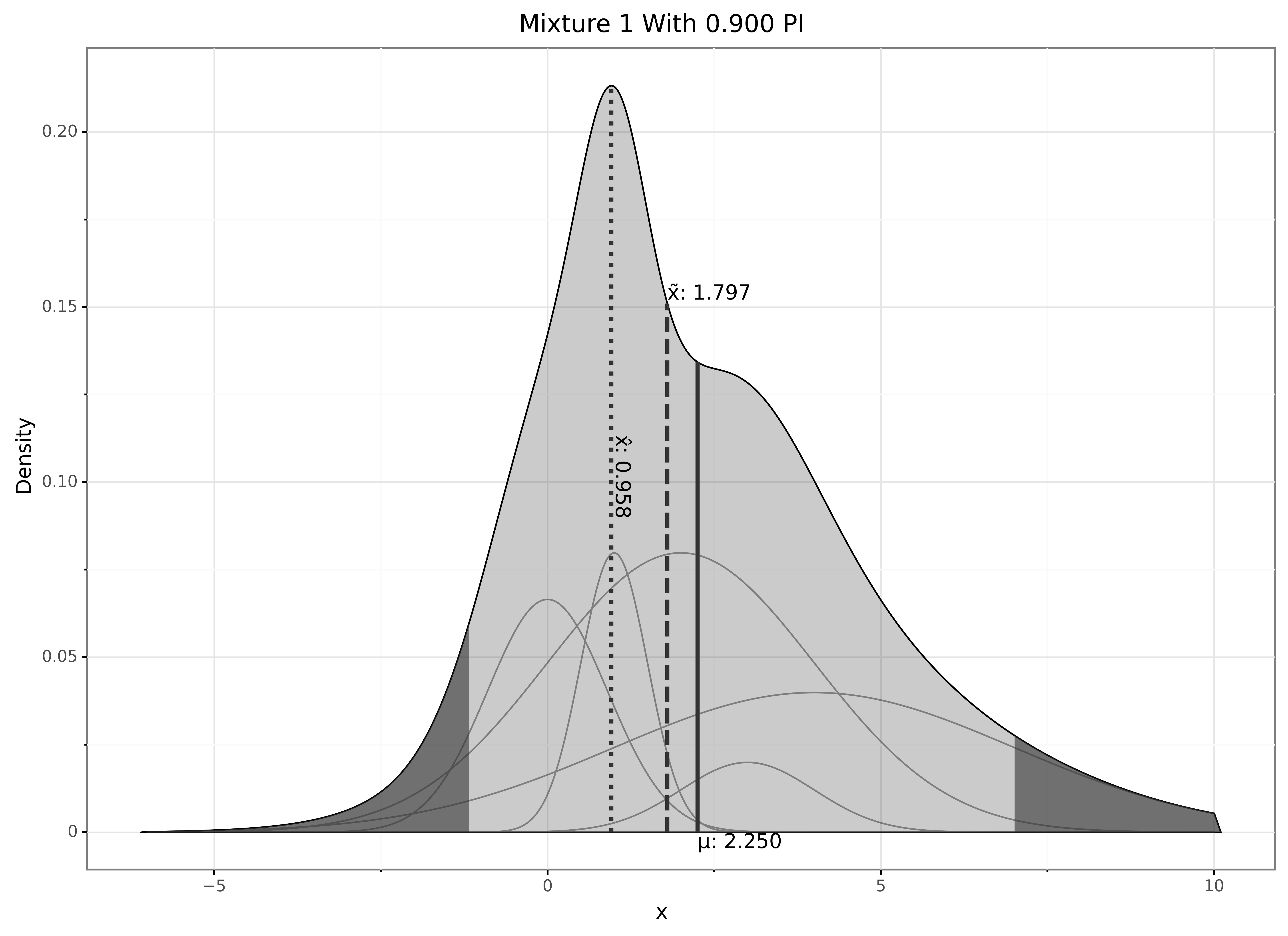
In addition to the standard distribution functions you can also gmix2.plot() one or more distributions.
>>> gmix.plot(
    weights[0],
    means[0],
    sigmas[0],
    mixture_names=['Mix1'],
    show_mean=True,
    show_median=True,
    show_mode=True,
    show_mixture=True,
    percent_interval=0.9)
The output of the plot is shown below.
The density of the full distribution is shaded in gray with a 90% probability interval indicated by the light gray region.
Each individual component of the mixture can also be plotted (show_mixture=True), which are the smaller curves in the shaded region.
The mean value (\(\mu\)) can be added to the plot and is also indicated by a solid vertical line.
The median value (\(\tilde{x}\)) can be added to the plot and is also indicated by a vertical dashed line.
The modes (\(\hat{x}\)) can be added to the plot and are also indicated by a vertical dotted line.
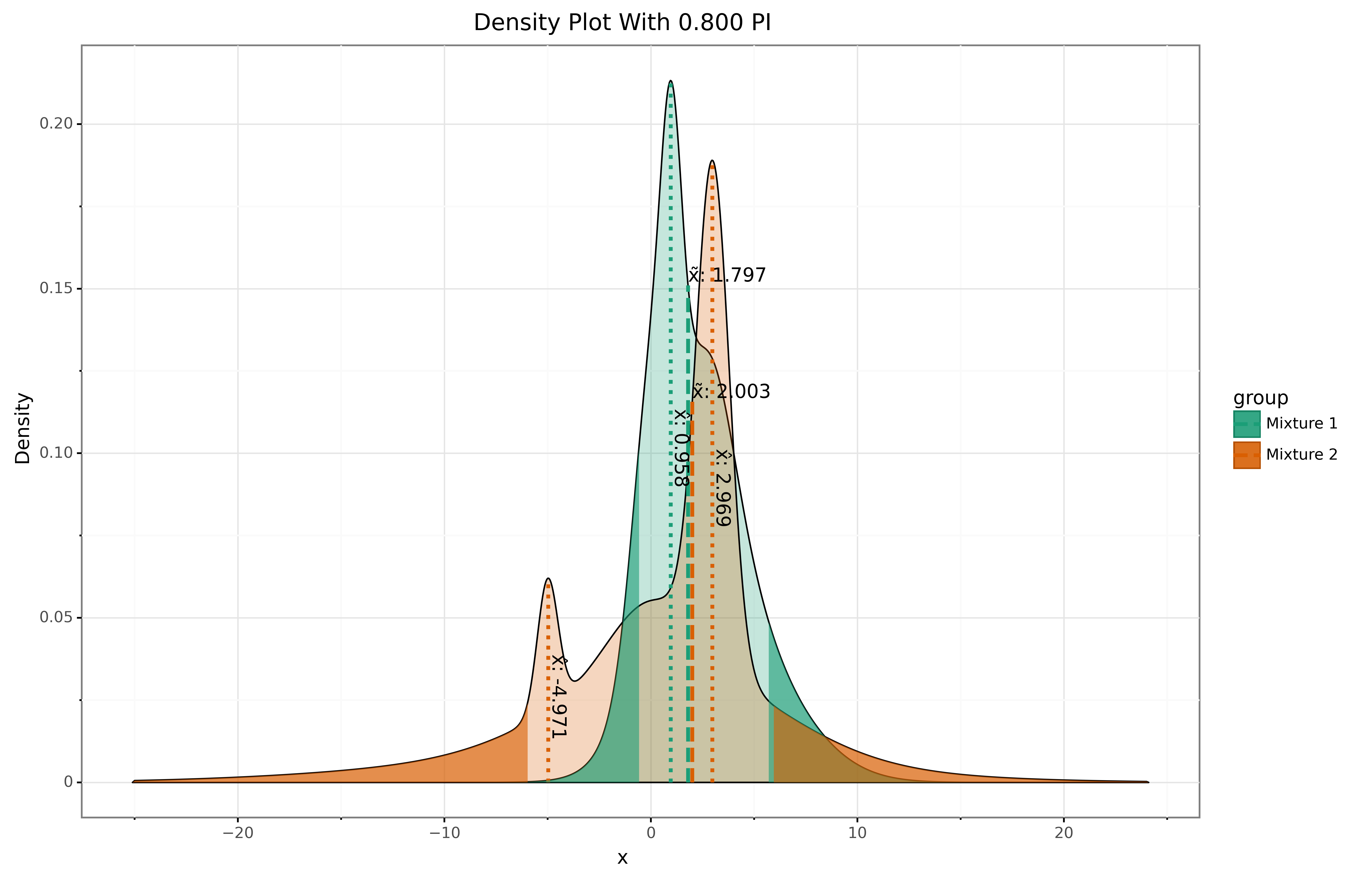
Here is another example with two mixtures plotted together.
>>> gmix.plot(
    weights,
    means,
    sigmas,
    row_names=['Mixture 1', 'Mixture 2'],
    show_median=True,
    show_mode=True,
    percent_interval=0.8)